曲线分析
采集好的曲线,默认情况采集好的曲线保存到当前Jupyter notebook所在的同级目录下的dataset文件夹下,其以时间戳格式命名,如:20250519101918.zarr。
我们使用scarr库对波形进行分析,其安装方式参考:SCARR安装
运行scarr进行分析
在Jupyter notebook中分别插入并执行如下代码,开始对这个曲线进行分析
定义波形文件路径
# 这里替换为你采集到的波形文件
trace_path = r'./dataset/20250519122059.zarr'
引入必要依赖
from scarr.engines.cpa import CPA as cpa
from scarr.file_handling.trace_handler import TraceHandler as th
from scarr.model_values.sbox_weight import SboxWeight
from scarr.container.container import Container, ContainerOptions
import numpy as np
执行分析
handler = th(fileName=trace_path)
model = SboxWeight()
engine = cpa(model)
container = Container(options=ContainerOptions(engine=engine, handler=handler), model_positions = [x for x in range(16)])
container.run()
查看结果
执行完上述代码后,曲线就应分析出密码。
查看分析出的密码结果
candidate = np.squeeze(engine.get_candidate()) # get_candidate 获取各个字节的密钥的计算结果
' '.join(f"{x:02x}" for x in candidate) # 打印计算出的密钥
其将打印出密钥

对应前面的波形采集章节,我们使用的密钥是11 22 33 44 55 66 77 88 99 00 aa bb cc dd ee ff,说明密钥已经成功的分析出来。
import random
import time
from cracknuts.cracker import serial

cmd_set_aes_enc_key = "01 00 00 00 00 00 00 10"
cmd_aes_enc = "01 02 00 00 00 00 00 10"

aes_key = "11 22 33 44 55 66 77 88 99 00 aa bb cc dd ee ff"
aes_data_len = 16

...
验证结果
我们可以验证下这个分析结果,执行下面的代码,检查第0个字节猜测密钥的相关性情况
result_bytes = np.squeeze(container.engine.get_result())
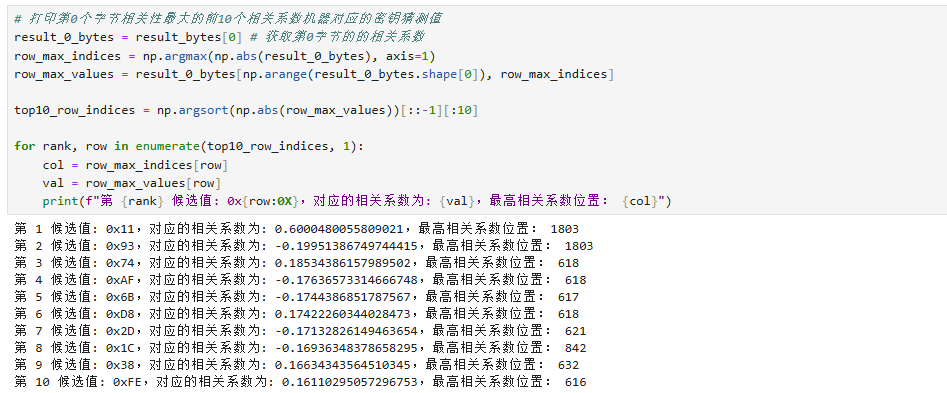
打印第0个字�节相关性最大的前10个相关系数机器对应的密钥猜测值
result_0_bytes = result_bytes[0] # 获取第0字节的的相关系数
row_max_indices = np.argmax(np.abs(result_0_bytes), axis=1)
row_max_values = result_0_bytes[np.arange(result_0_bytes.shape[0]), row_max_indices]

top10_row_indices = np.argsort(np.abs(row_max_values))[::-1][:10]

for rank, row in enumerate(top10_row_indices, 1):
    col = row_max_indices[row]
    val = row_max_values[row]
    print(f"第 {rank} 候选值: 0x{row:0X},对应的相关系数为: {val},最高相关系数位置: {col}")`
上述代码将打印出像关系最大的前是个猜测密钥:
提示
你那里打印出的和是不一样的,只要第一个相同就是正确的
此处可以看到第0字节0x11的相关性最大,说明上面的密钥结果没有问题。
此外还可以波形查看其相关性信息,执行如下代码查看:
定义一个绘制相�关性波形的函数
import numpy as np
import matplotlib.pyplot as plt

def plot_correlation_peaks(bytes_index, the_key):

    x = np.arange(0, 5000)

    fig, ax = plt.subplots(figsize=(30, 4))

    for i in range(256):
        if i == the_key:
            continue
        ax.plot(x, result_bytes[bytes_index, i, :5000], color='gray', linewidth=0.5, alpha=0.3)

    ax.plot(x, result_bytes[bytes_index, the_key, :5000], color='red', linewidth=1.0)

    ax.grid(True, linestyle='--', alpha=0.3)
    plt.tight_layout()

    plt.show()
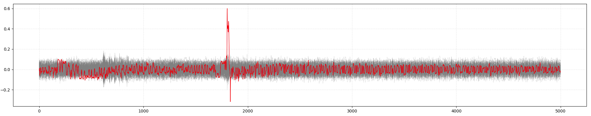
绘制第0字节的256个密钥猜测下的相关系数曲线
plot_correlation_peaks(0, 0x11)
将绘制如下的图形,可以看出正确密钥对应的相关系数曲线存在最明显的尖峰:
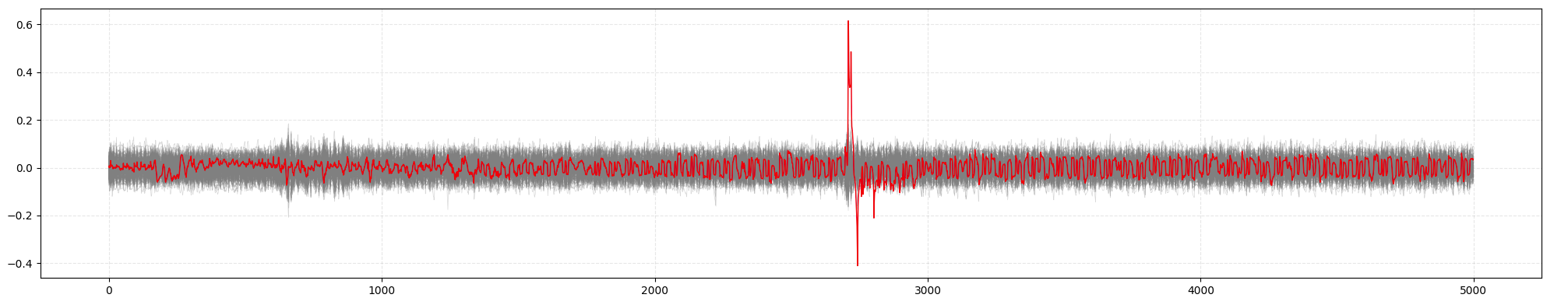
同样也可以绘制其他字节的猜测密钥
绘制第1字节的256个密钥猜测下的相关系数曲线
plot_correlation_peaks(1, 0x22)
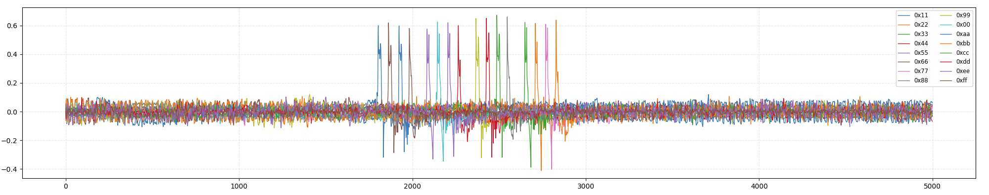
把所有16个字节正确密钥对应的相关系数曲线画出来,以便观察它们的时间点。
16个字节的争取密钥的相关系数曲线
import matplotlib.pyplot as plt

x = np.arange(0, 5000)

fig, ax = plt.subplots(figsize=(30, 4))

ax.plot(x, result_bytes[0, 0x11, :5000], linewidth=1.0, label='0x11')
ax.plot(x, result_bytes[1, 0x22, :5000], linewidth=1.0, label='0x22')
ax.plot(x, result_bytes[2, 0x33, :5000], linewidth=1.0, label='0x33')
ax.plot(x, result_bytes[3, 0x44, :5000], linewidth=1.0, label='0x44')
ax.plot(x, result_bytes[4, 0x55, :5000], linewidth=1.0, label='0x55')
ax.plot(x, result_bytes[5, 0x66, :5000], linewidth=1.0, label='0x66')
ax.plot(x, result_bytes[6, 0x77, :5000], linewidth=1.0, label='0x77')
ax.plot(x, result_bytes[7, 0x88, :5000], linewidth=1.0, label='0x88')
ax.plot(x, result_bytes[8, 0x99, :5000], linewidth=1.0, label='0x99')
ax.plot(x, result_bytes[9, 0x00, :5000], linewidth=1.0, label='0x00')
ax.plot(x, result_bytes[10, 0xaa, :5000], linewidth=1.0, label='0xaa')
ax.plot(x, result_bytes[11, 0xbb, :5000], linewidth=1.0, label='0xbb')
ax.plot(x, result_bytes[12, 0xcc, :5000], linewidth=1.0, label='0xcc')
ax.plot(x, result_bytes[13, 0xdd, :5000], linewidth=1.0, label='0xdd')
ax.plot(x, result_bytes[14, 0xee, :5000], linewidth=1.0, label='0xee')
ax.plot(x, result_bytes[15, 0xff, :5000], linewidth=1.0, label='0xff')

ax.grid(True, linestyle='--', alpha=0.3)
ax.legend(loc='upper right', fontsize='small', ncol=2)

plt.tight_layout()

plt.show()
从中可以看到16个字节密钥相关性系数的情况:
至此,恭喜你,你已经完成的CrackNuts的基本使用,更多功能和使用教程可参看其他章节。