Host Usage Guide

The host is developed in Python and communicates with the device via TCP protocol. It is recommended to use the host in a Jupyter environment to operate the device, which allows you to use the device control panel provided by the host to reduce code editing and view the effect of device parameter configuration in real time through the oscilloscope panel.

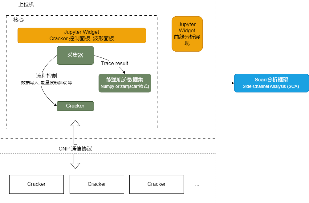
The overall architecture of the host is shown below:

For API documentation of the host SDK, visit https://cracknuts.readthedocs.io/zh-cn/stable/.

In the host, Cracker represents the device, and Acquisition represents the acquisition process. The host can control the device and collect data around these two modules.

Command Line Tools

After installing CrackNuts, the console provides the cracknuts command, which offers the following Jupyter shortcut commands:

1. Start Jupyter lab

   cracknuts lab
2. Open tutorials

   cracknuts tutorials
3. Create a new notebook

   cracknuts create -t [template name] -n [new notebook name]
4. Global configuration

   cracknuts config set lab.workspace  # Configure the default workspace directory for cracknuts lab

Basic Usage of the Host

After successful installation, you can control the device via Python. For example, you can directly access and configure the device through the Python console:

1. Start the Python environment:
   If you installed CrackNuts via the quick install method, you can start the CrackNuts environment using the shortcut icon. If installed by other means, choose the appropriate way to enter a Python environment with CrackNuts dependencies.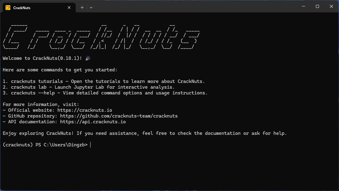

   

2. Connect to the device and configure Nut voltage

   

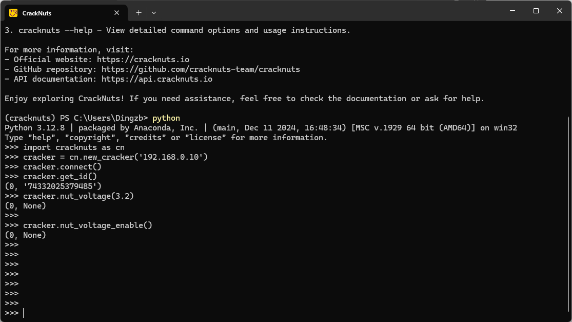
   The above code is explained as follows:

   # Import cracknuts
   >>> import cracknuts as cn
   # Create a Cracker object via the quick entry function
   >>> cracker = cn.new_cracker('192.168.0.211')
   # Connect to the device
   >>> cracker.connect()
   # Get device ID, used here to verify connection status. This is a simple and effective way to verify correct device connection.
   >>> cracker.get_id()
   (0, '74332025379485') # This is the return format of CrackNuts host API: the first element of the tuple is the function execution status, 0 means success, others mean failure; the second element is the returned data, here the device ID (S/N). For interfaces without return data, it is None.
   # Configure Nut device voltage to 3.2V
   >>> cracker.nut_voltage(3.2)
   (0, None) 
   # Enable Nut. The Nut board with default stm32 103 should light up.
   >>> cracker.nut_voltage_enable()
   (0, None)
   >>>

   This completes the simplest host control. For more configurations, refer to the API documentation.

Acquisition Process

In the "Quick Start" section, you may have noticed that when using CrackNuts for waveform acquisition, you only need to control the Nut's actions to complete the energy waveform acquisition. This is because CrackNuts has designed a simplified acquisition process to reduce operational complexity and allow users to focus on core processes such as Nut encryption.

This acquisition process is managed by the Acquisition class, i.e., the acq object created before using the control panel. This object implements key steps such as command sending, encrypted data saving, and energy trace saving, and reserves init and do stages for users to insert custom logic. Through this process, users can achieve the following:

• Configure parameters via GUI, support real-time waveform display for easy device adjustment;
• Automatically save configuration parameters for easy experiment reproduction;
• Automatically save acquired trace data for subsequent analysis.

The structure of the acquisition process is shown below:

The corresponding flowchart for Cracker and Nut is shown below:

In the diagram, CrackNuts is the host software, Cracker is the test device, Nut is the target, and Wave represents the side-channel signal. Users need to implement two functions: init() and do(). The init() function is executed once at the start of the acquisition process, while the do() function is called in a loop. In these functions, users can write specific command logic, send it to Nut via Cracker, and receive data returned by Nut, which Cracker then forwards to the CrackNuts host program. After init() completes, CrackNuts automatically sends the osc_single() command to Cracker, setting it to "ready to acquire trace" mode. The trigger conditions can be configured via the host interface or commands, supporting parameters such as signal source (A/B channel), trigger target (e.g., Nut), communication protocol, etc. During do() execution, Cracker monitors trigger conditions in real time and acquires waveform data immediately once triggered. After do() completes, CrackNuts automatically determines if acquisition was successful: if triggered, it reads and saves the acquired data from Cracker.

The creation of Acquisition in the Quick Start section is this acquisition process:

import random
import time
from cracknuts.cracker import serial

cmd_set_aes_enc_key = "01 00 00 00 00 00 00 10"
cmd_aes_enc = "01 02 00 00 00 00 00 10"

aes_key = "11 22 33 44 55 66 77 88 99 00 aa bb cc dd ee ff"
aes_data_len = 16

sample_length = 1024 * 20

def init(c):
    cracker.nut_voltage_enable()
    cracker.nut_voltage(3.4)
    cracker.nut_clock_enable()
    cracker.nut_clock_freq('8M')
    cracker.uart_enable()
    cracker.osc_sample_clock('48m')
    cracker.osc_sample_length(sample_length)
    cracker.osc_trigger_source('N')
    cracker.osc_analog_gain('B', 10)
    cracker.osc_trigger_level(0)
    cracker.osc_trigger_mode('E')
    cracker.osc_trigger_edge('U')
    cracker.uart_config(baudrate=serial.Baudrate.BAUDRATE_115200, bytesize=serial.Bytesize.EIGHTBITS, parity=serial.Parity.PARITY_NONE, stopbits=serial.Stopbits.STOPBITS_ONE)

    time.sleep(2)
    cmd = cmd_set_aes_enc_key + aes_key
    status, ret = cracker.uart_transmit_receive(cmd, timeout=1000, rx_count=6)

def do(c):

    plaintext_data = random.randbytes(aes_data_len)
    tx_data = bytes.fromhex(cmd_aes_enc.replace(' ', '')) + plaintext_data
    status, ret = cracker.uart_transmit_receive(tx_data, rx_count= 6 + aes_data_len, is_trigger=True)
    
    return {
        "plaintext": plaintext_data,
        "ciphertext": ret[-aes_data_len:],
        "key": bytes.fromhex(aes_key)
    }

acq = cn.new_acquisition(cracker, do=do, init=init)

The required parameters for new_acquisition are as follows:

• cracker: The Cracker target managed by the Acquisition process
• do: The user's specific encryption logic function, which must return data to be saved in the waveform file
• init: Preparations before energy trace acquisition, such as basic configuration

Similarly, in the control panel (see later sections for introduction to the control panel in Jupyter), there are richer process control parameters:

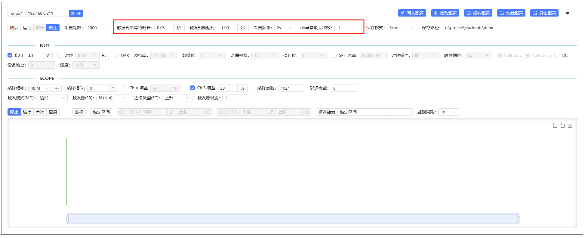
Their meanings are as follows (refer to the flowchart above for better understanding). If you are not familiar with the overall process, it is not recommended to modify these parameters:

• Trigger wait duration: Interval between each is_trigger check
• Trigger timeout: If the device does not detect a trigger within this time, the acquisition round is considered failed
• Acquisition frequency: In test mode, how often to perform encryption operations on the device
• Maximum do exceptions: The number of errors allowed in the user's do function code, default -1 means no errors allowed

Other functions in the process management area of the control panel are as follows:

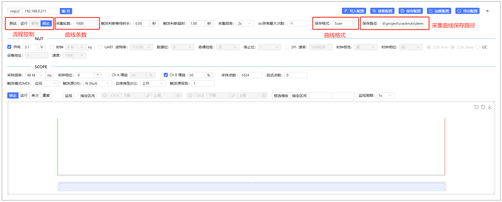
• Process status control:
  • Test: Only perform data encryption and energy trace operations, do not save waveform files
  • Run: Perform complete data encryption, energy acquisition, and file saving
  • Pause: Pause the current test or run process
  • Stop: Stop the current test or run process
• Acquisition rounds: Number of traces to acquire, i.e., how many times to execute the do function
• Save format: Format for saving trace files, default is scarr, optional numpy
• Save path: Folder for saving trace files, files are named by timestamp and saved in this directory

Other functions of the CrackNuts panel can be found in later chapters.

Using CrackNuts Host in Jupyter

In addition to using CrackNuts in the Python console and scripts, you can also use it in the Jupyter environment, which is our recommended method. In Jupyter, we provide a more concise GUI control panel for device control and data display.

We also provide the simple command cracknuts lab to start a Jupyter environment.

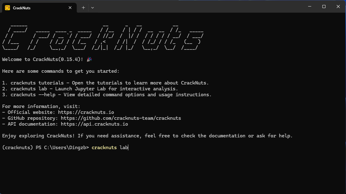
Use the above command to start a Jupyter lab environment, then create a Jupyter Notebook to begin device control.

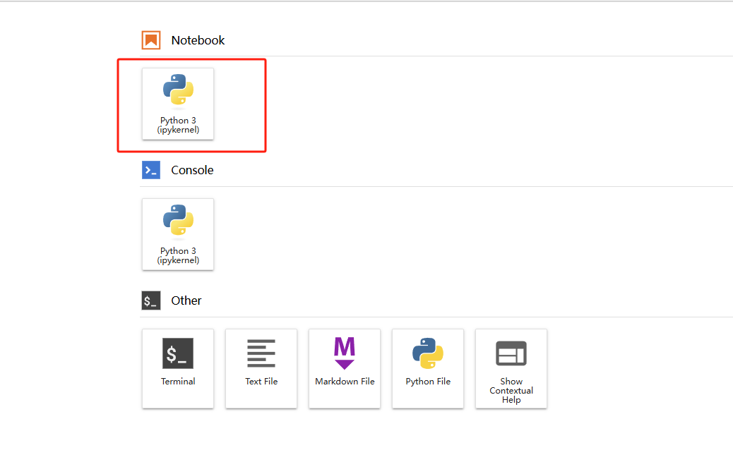
Enter the following code in two cells in the new Notebook to open the device control panel:

Cell 1

import cracknuts as cn

cracker = cn.new_cracker('192.168.0.10')
cracker.connect()
cracker.get_id()

Cell 2

cracker.nut_voltage(3.1)
cracker.nut_voltage_enable()

After entering the code in each cell, execute it to complete the operation. (Use Ctrl+Enter to execute, or Shift+Ctrl to execute and automatically activate the next cell.)

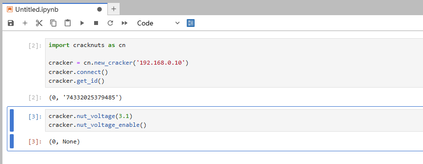
After executing the above steps, you can also complete Nut voltage configuration and enabling.

Jupyter Control Panel Component

In Jupyter, you can use the device control panel to control the device. Execute the following code to open the device control panel:

# Create an empty acquisition process control object
acq = cn.new_acquisition(cracker)
# Show panel
cn.panel(acq)

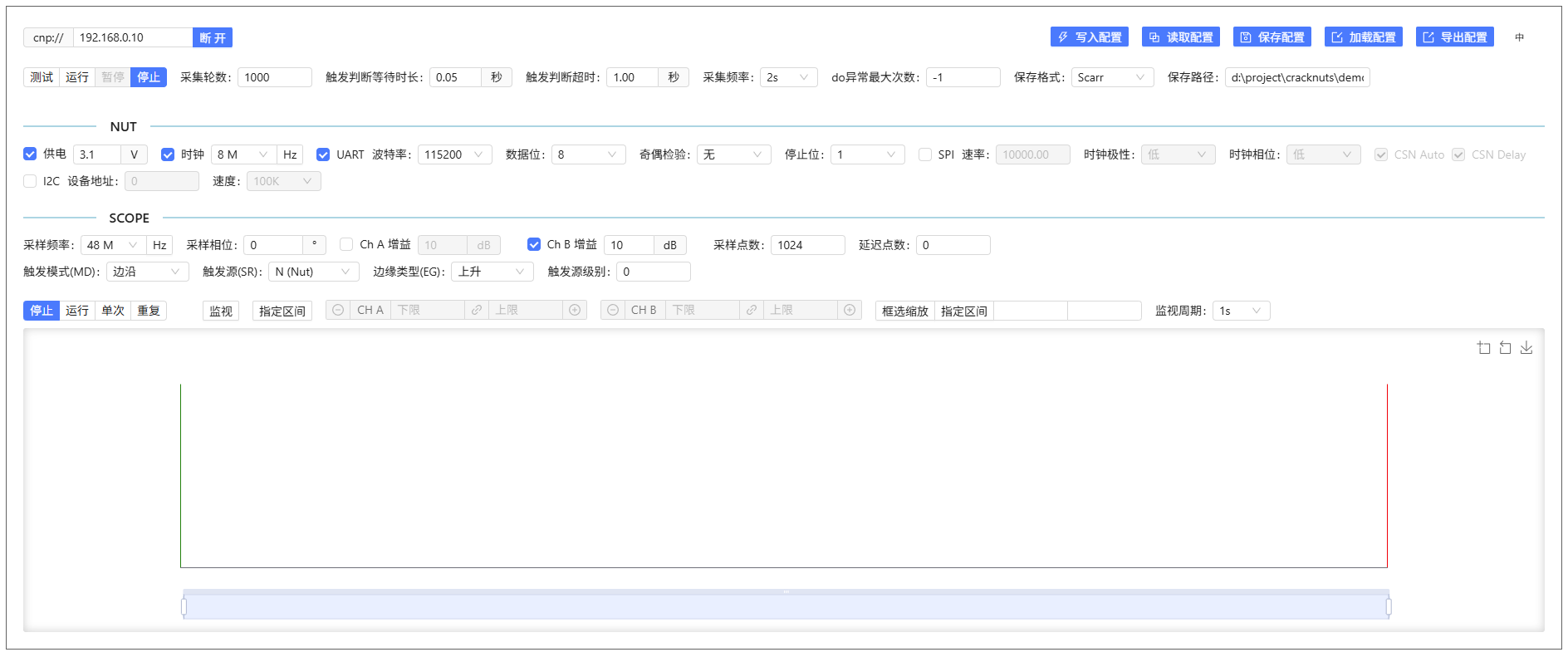
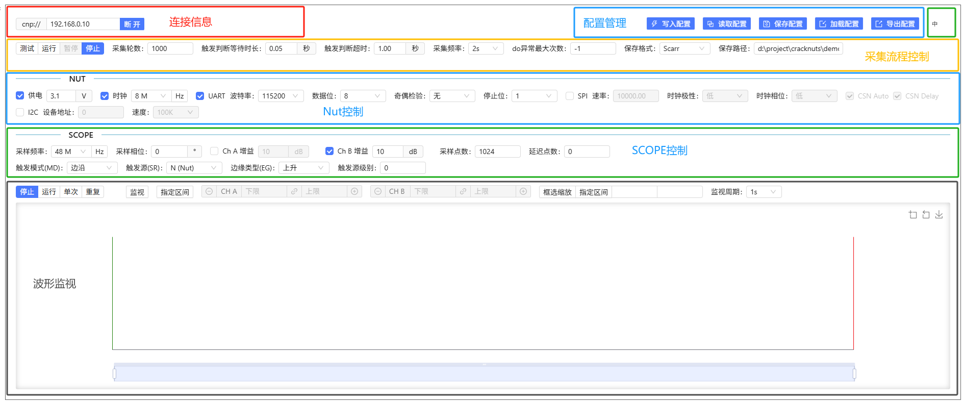
The device control panel integrates four major modules: acquisition process management, NUT management, SCOPE management, and model display, which respectively implement energy trace acquisition management, NUT target board control, Cracker acquisition board control, and waveform display.

Waveform Display

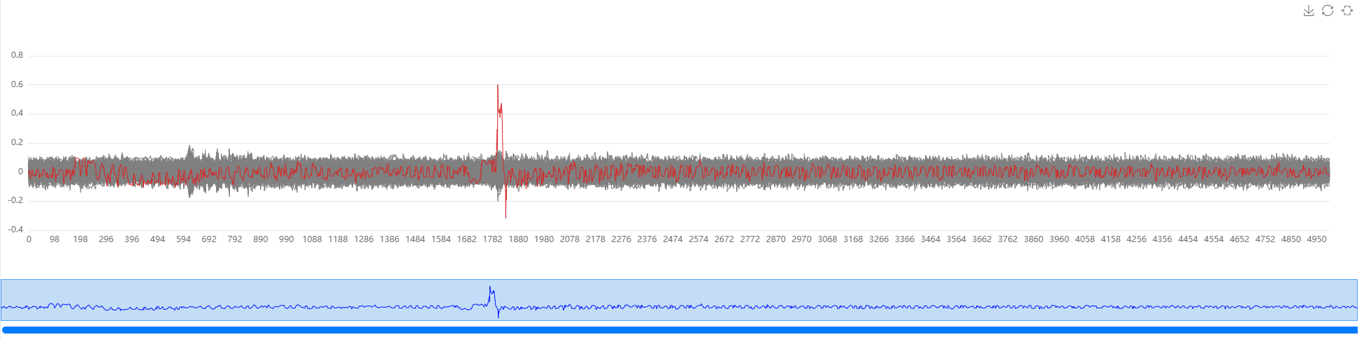
The CrackNuts host provides a Jupyter widget for displaying acquired waveforms, which efficiently supports zooming and other operations.

For example, you can open a CrackNuts-acquired waveform dataset:

import cracknuts as cn
from cracknuts.trace import ZarrTraceDataset

trace_path = r'./dataset/20250519122059.zarr'
# Load scarr format dataset
ds = ZarrTraceDataset.load(trace_path)

pt = cn.panel_trace()
pt.set_trace_dataset(ds)
pt

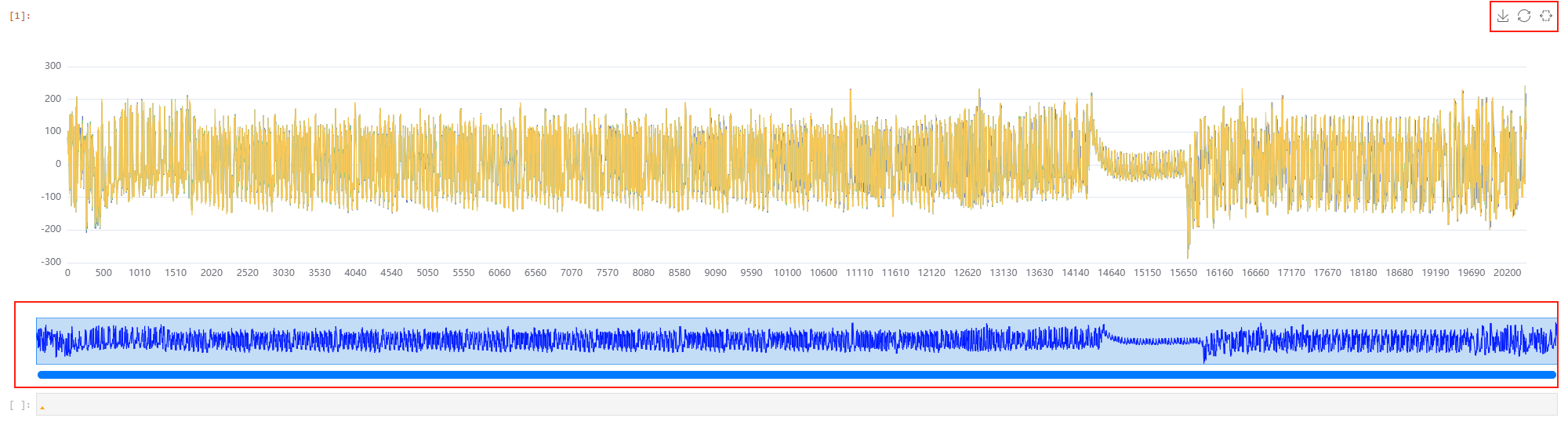
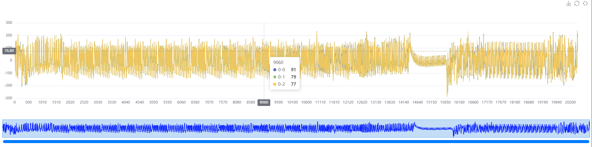
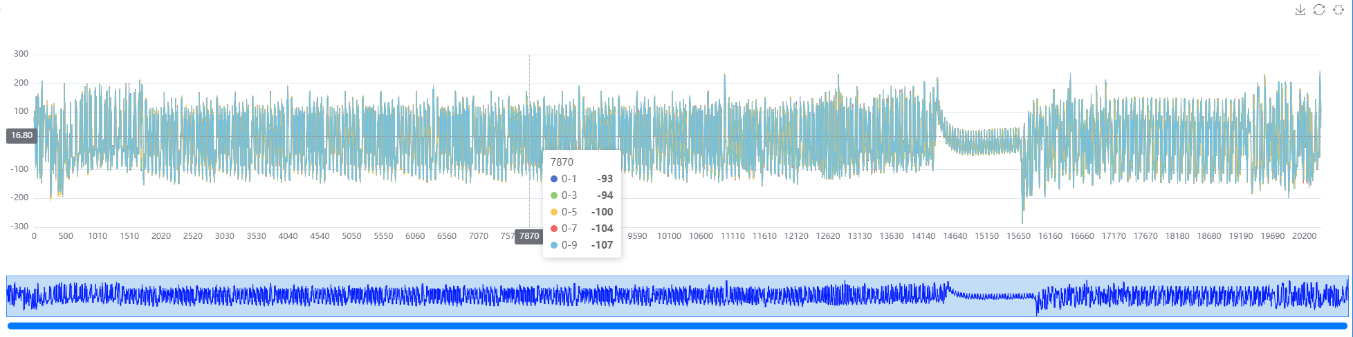
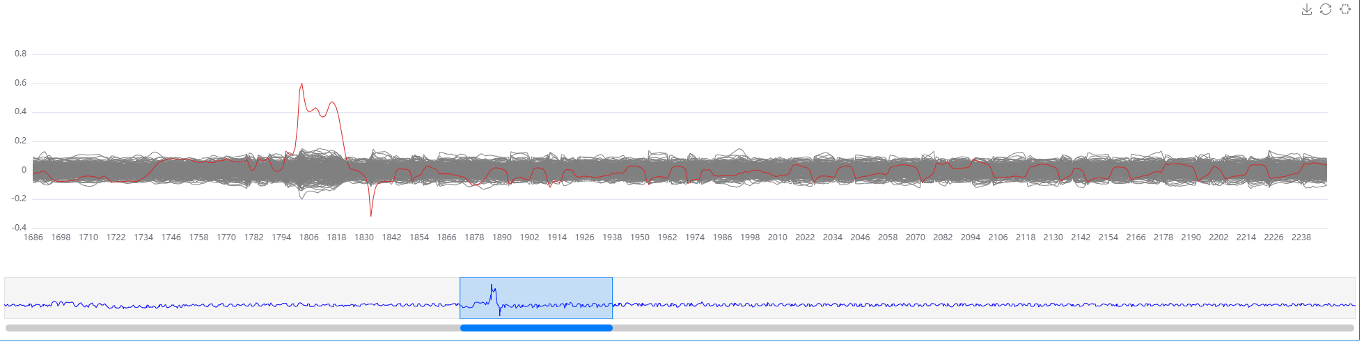
In the figure above, the upper control area allows downloading, resetting zoom, and enabling selection zoom. The lower zoom indicator area shows the current zoom interval and allows dragging the zoom interval.

Clicking on the waveform with the mouse displays the coordinate and value information at the current position.

In addition to mouse zoom control in this Jupyter widget, you can also control zoom precisely via code:

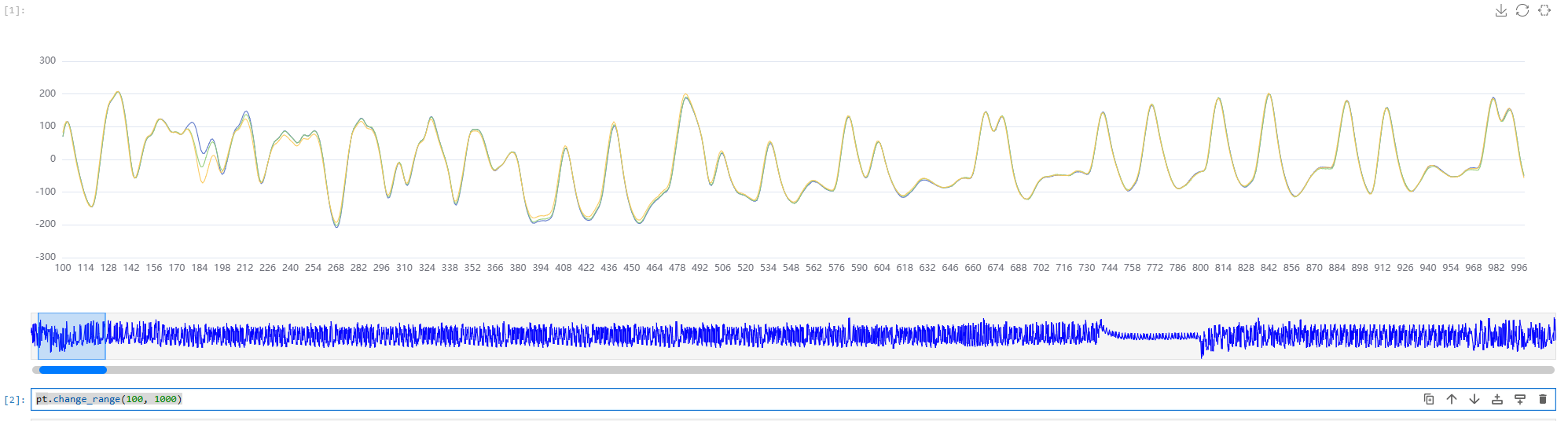
# Specify zoom interval by index
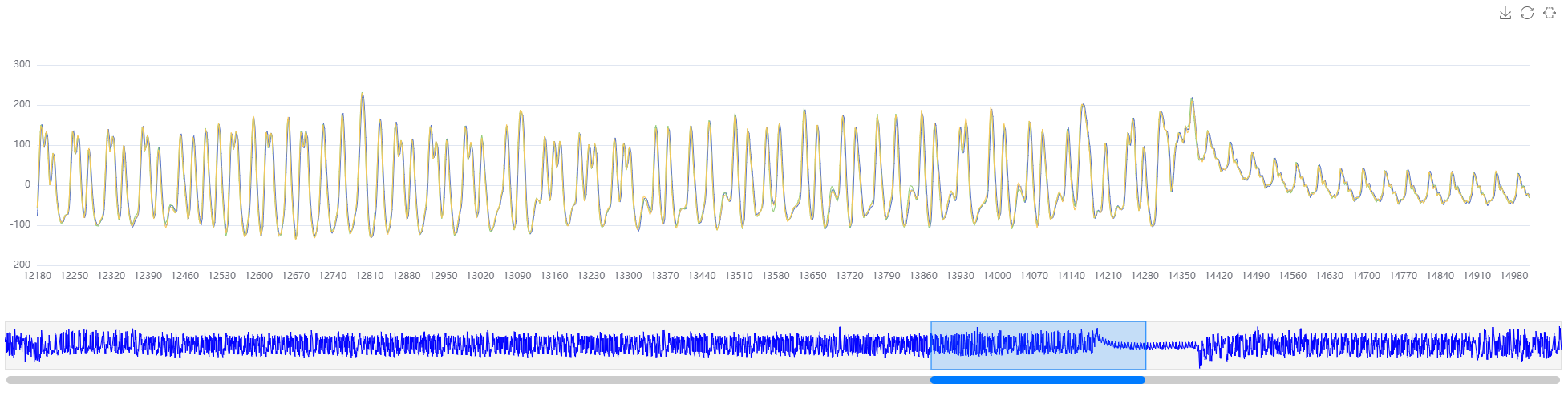
pt.change_range(100, 1000)

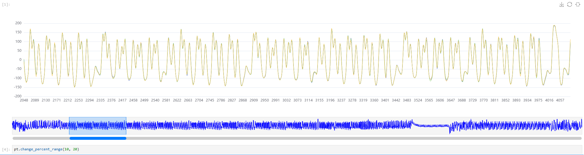
# Specify zoom interval by percentage
pt.change_percent_range(10, 20)

Since the acquired data points are usually large, only the first three traces are displayed by default. To switch traces, use the show_trace property. show_trace is a property of TracePanelWidget and supports slicing. The first slice is the channel index, the second is the trace index.

pt.show_trace[0, :10] # First 10 traces of channel 0

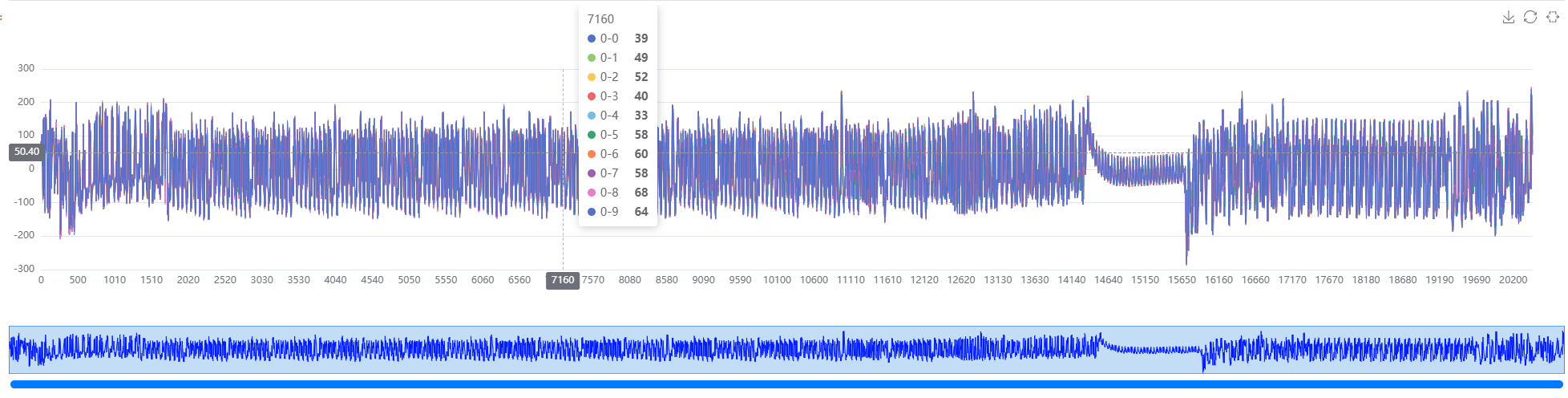
pt.show_trace[0, 1:10:2] # Channel 0, traces 1 to 10, step 2

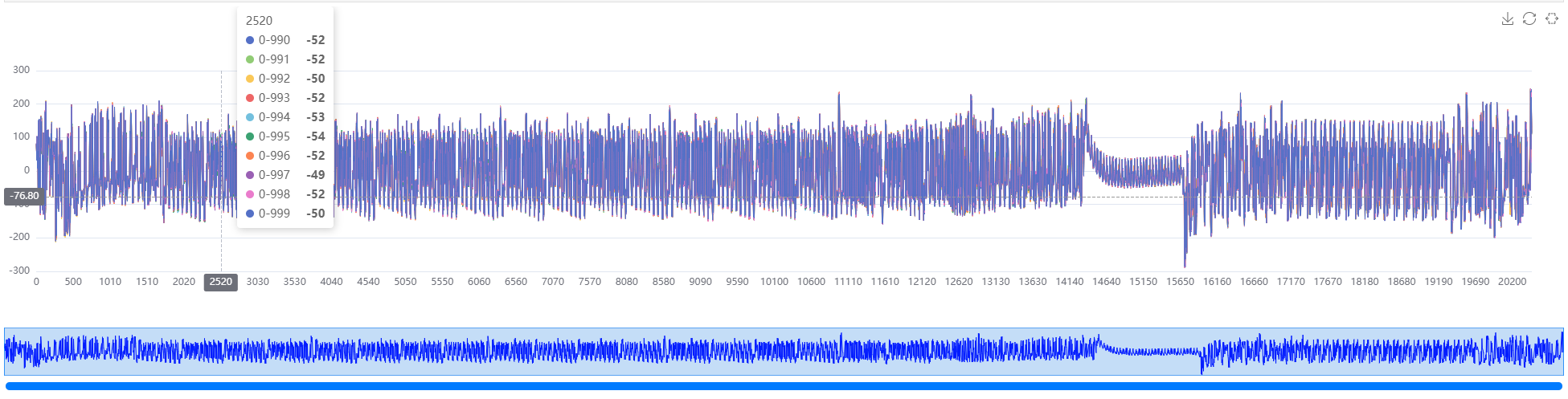
pt.show_trace[0, -10:] # Last 10 traces

In addition to opening CrackNuts-acquired dataset files, you can also directly open numpy arrays for intermediate analysis. The array should be one- or two-dimensional, with the first dimension as traces and the second as data points, for example:

import numpy as np

y = np.random.randint(100, size=(10, 1000)) # Generate a 2D array

pt.set_numpy_data(y)

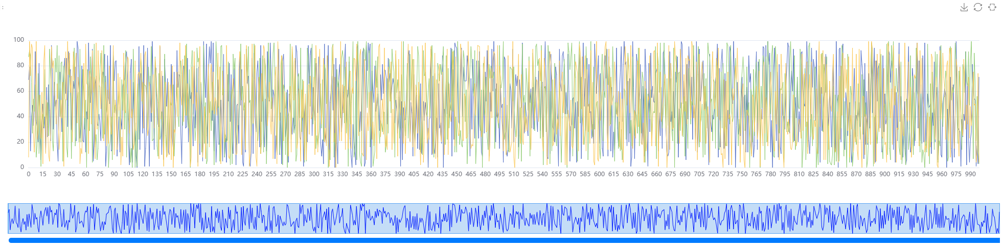
The above is a numpy example with random numbers. In most cases, after curve analysis, you can check the correlation.

# Detailed curve analysis process omitted, refer to the Quick Start section
from scarr.engines.cpa import CPA as cpa
from scarr.file_handling.trace_handler import TraceHandler as th
from scarr.model_values.sbox_weight import SboxWeight
from scarr.container.container import Container, ContainerOptions
import numpy as np

handler = th(fileName=trace_path) 
model = SboxWeight() 
engine = cpa(model)
container = Container(options=ContainerOptions(engine=engine, handler=handler), model_positions = [x for x in range(16)])
container.run()

result_bytes = np.squeeze(container.engine.get_result())

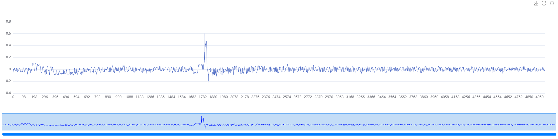
correlation_best = result_bytes[0, 0x11, :5000] # Correlation of the 0x11-th key guess for the 0-th byte

pt.set_numpy_data(correlation_best)

Of course, you can also view all data in the correlation matrix and highlight the curve of the guessed key (not recommended, as our component is interactive and the correlation matrix is large, which may cause the page to freeze. For static display, refer to the Quick Start section).

correlation = result_bytes[0, :, :5000] # Get correlation curves for all key guesses of the 0-th byte
pt.set_numpy_data(correlation)
pt.show_all_trace() # Show all curves
pt.highlight(0x11) # Highlight

Jupyter Notebook Configuration

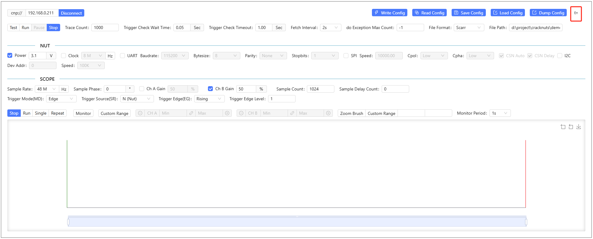
After using the control panel in Jupyter, you can use the configuration feature to save, export, import, and write the current panel configuration to the device, or read the device's current configuration into the panel.

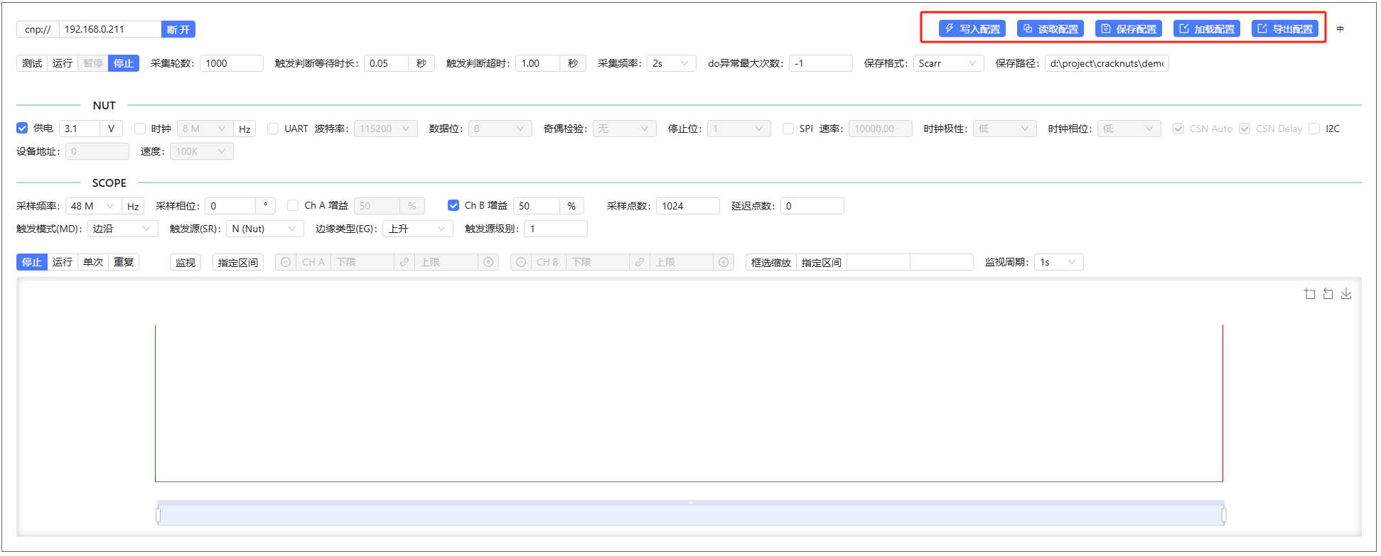
The difference between Save Configuration and Export Configuration is that the former saves the current configuration to a file associated with the Jupyter Notebook, and the next time you open the device control panel in that notebook, it automatically loads the configuration. Exporting configuration exports to a configuration file, which users can load as needed via Load Configuration.

warning

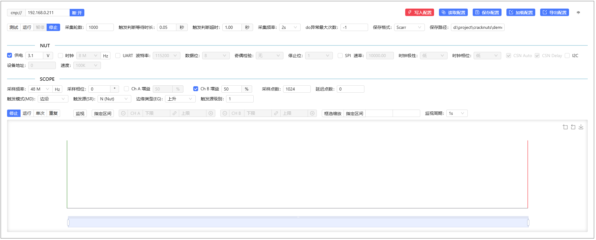
By default, device configuration via code is synchronized to the control panel. However, if the panel loads a configuration file (either the notebook-associated or an external configuration via Load Configuration) and it differs from the device configuration, the panel will prompt by turning the Write Configuration button red. At this time, device configuration via code will not sync to the panel until you write the configuration to the device via the button.

Language Switching

The control panel defaults to English on first use. You can switch languages via the button in the upper right corner, which affects all Jupyter Notebooks.

Jupyter Default Workspace Configuration

The Jupyter lab instance started via cracknuts lab can be configured with a default workspace using the following command, ensuring that the workspace is used regardless of the current directory.

cracknuts config set lab.workspace

Log Configuration

By default, CrackNuts logs are printed to the current console, or to the cell output in Jupyter, which helps users debug and troubleshoot.

Log Level Configuration

CrackNuts logs are warning level by default, printing only necessary warnings and errors. For more detailed information such as sent data, change the log level to info:

from cracknuts import logger
logger.set_level('info')

Or for even more detail, set the log level to debug, but note that this will print a lot of information:

from cracknuts import logger
logger.set_level('debug')

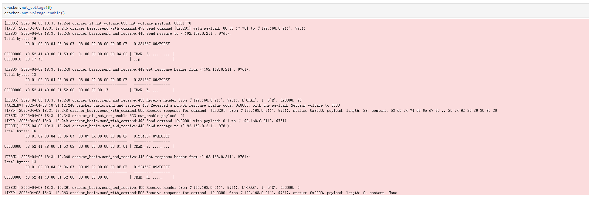
Log Output Location Configuration

Sometimes, especially during energy trace acquisition, there can be a lot of log output. Printing logs to the console or Jupyter Notebook can make the page very long and hard to use. You can redirect logs to a file and check them with other tools:

from cracknuts import logger
logger.handler_to_file(r"d:\a.log")

After configuration, open the log file with any text editor:

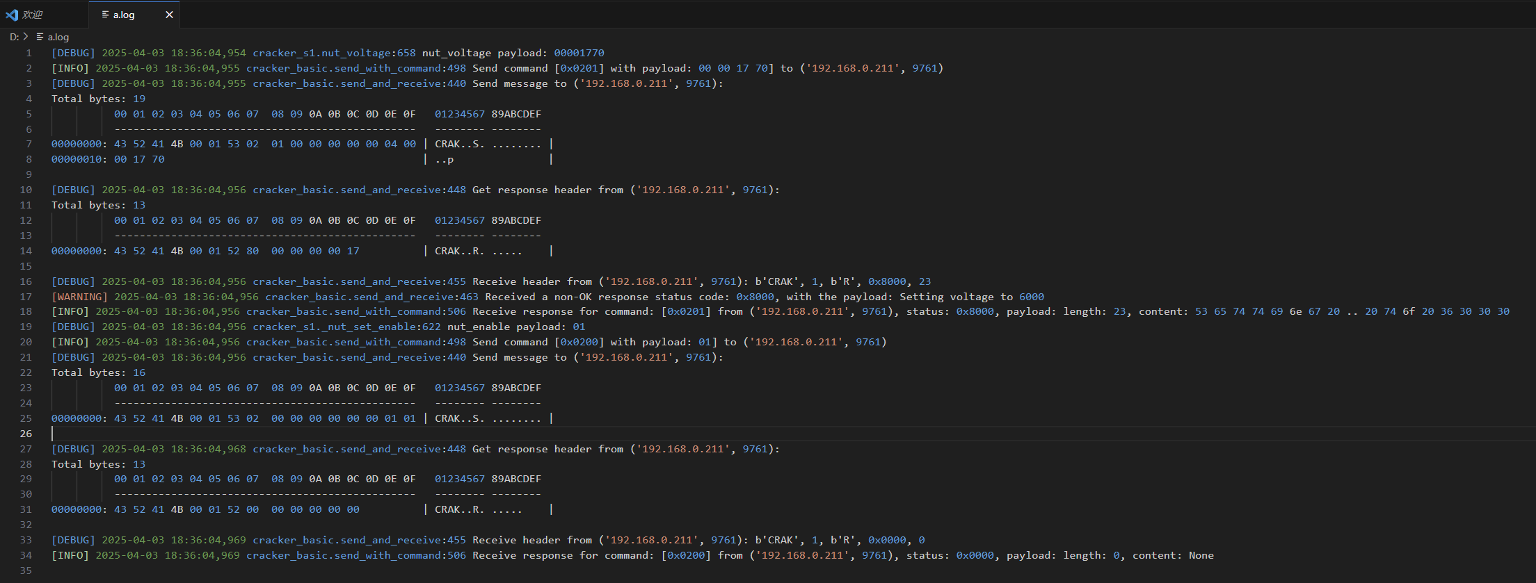
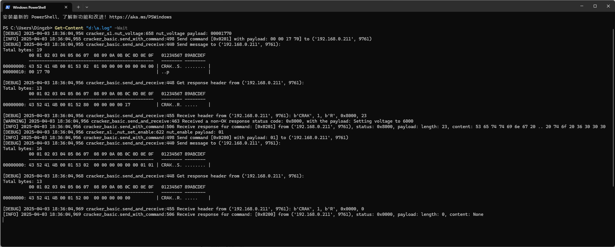
Linux or MacOS users can monitor logs in real time with tail -f. Windows users can use Get-Content "d:\a.log" -Wait in Powershell for a similar effect.

Change Cracker IP Address

If you connect the Cracker to an existing Ethernet, the IP network must be 192.168.0.0/24. If your network is not in this range, you need to change the Cracker's IP. First, connect directly to the device, then use the host SDK to change the IP.

Open the CrackNuts environment, start Python, and execute the following code to change the IP:

import cracknuts as cn
s1 = cn.new_cracker('192.168.0.10')
s1.connect()
s1.get_operator().set_ip('192.168.0.251', '255.255.255.0', '192.168.0.1')  # Change IP, mask, and gateway to match your target network

After successful execution, the Cracker device's display will show the new